
Python has become one of the most popular programming languages for data analysis, and for good reason. Its wide range of libraries and analytical tools makes it a powerful choice for researchers and professionals looking to extract valuable insights from their data. In this article, we will explore Python’s capabilities in data analysis through an exciting case study in the field of monetary policy.
The Case Study: Analyzing the Federal Reserve’s Monetary Policy
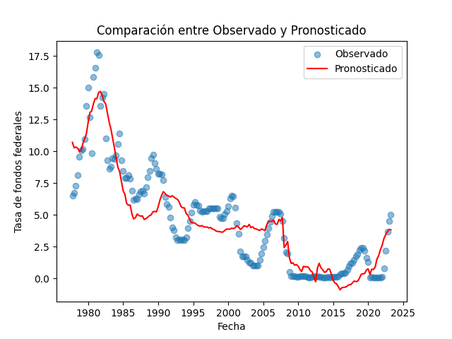
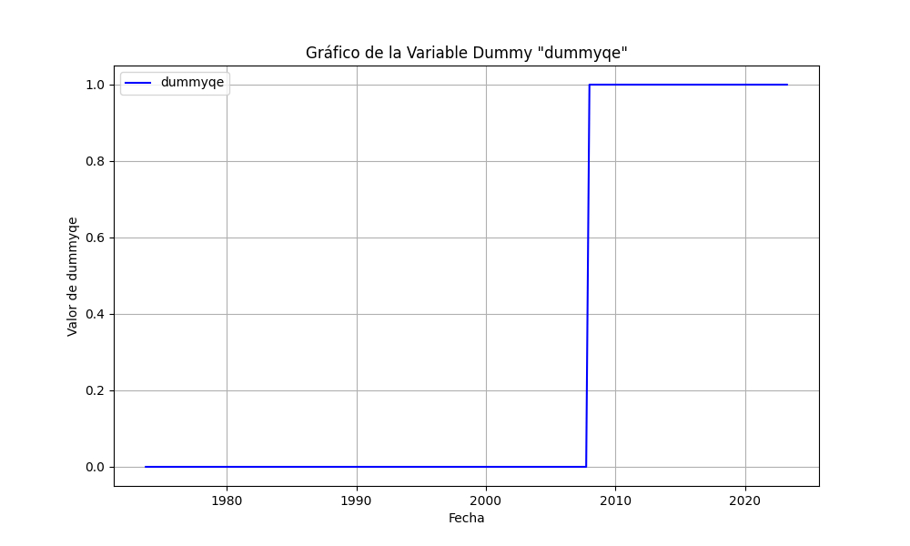
In this case study, we have used Python to analyze a dataset that addresses the monetary policy of the United States Federal Reserve. We conducted a series of essential statistical tests to assess the quality and robustness of a robust linear regression model (RLM) that relates the federal funds rate to productivity growth rates (Deltapr) and inflation (Deltacpi), along with a dummy variable representing a significant event associated with the introduction of Quantitative Easing (dummyqe).
Python’s Marvels in Action
We utilized Python to perform a variety of tests and analyses, showcasing the capabilities of this language:
- Cointegration Test: We began by assessing the cointegration relationship between the variables using Python. This test is crucial in determining whether there is a long-term relationship between the variables and if they can be used in a regression.
- Multicollinearity Test: We used Python to evaluate multicollinearity among the independent variables. This test is vital to ensure that our explanatory variables are not highly correlated, which could affect the model’s interpretation.
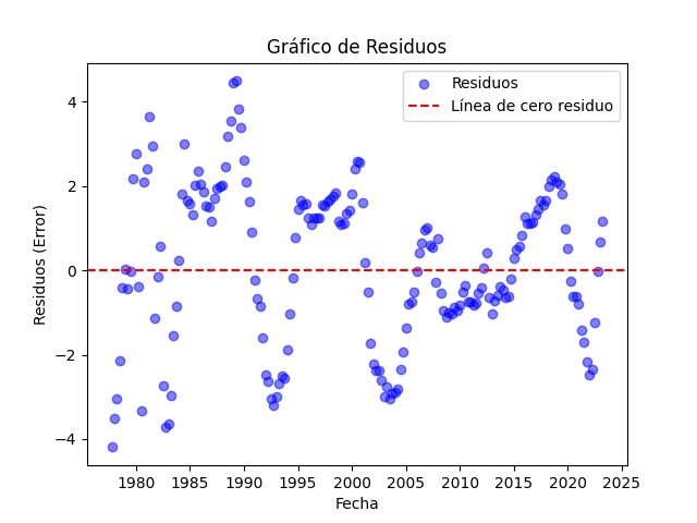
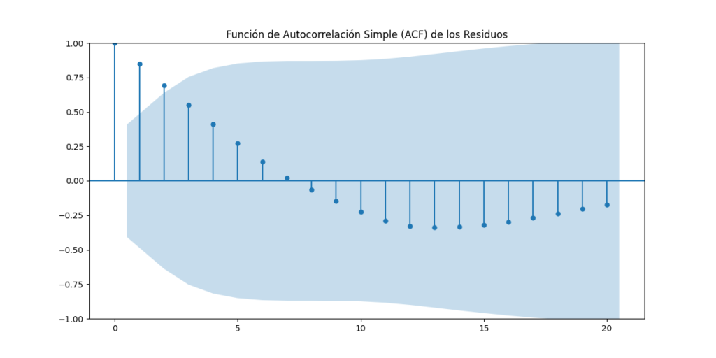
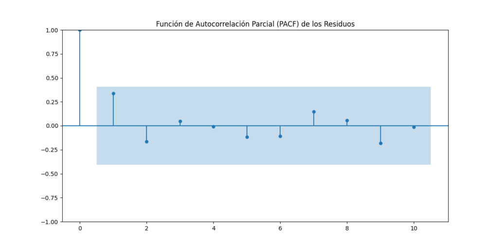
- Autocorrelation Test: We employed Python to examine the autocorrelation of the model’s residuals. This allows us to identify any patterns in the residuals and ensure that there are no unaccounted temporal dependency structures in the model.
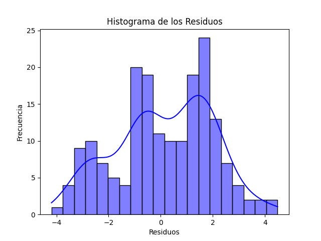
- Normality Test: We used Python to check the normality of the residuals. Normality of residuals is an important assumption of linear regression, and this test helps confirm its validity.
- Homoscedasticity Test: In addition to the aforementioned tests, we also explored the homoscedasticity of the model’s residuals in Python. Homoscedasticity refers to the equality of variance of the residuals across all levels of the independent variables. By checking for homoscedasticity, we ensure that the model’s errors are constant under all conditions, which is crucial for the validity of inferences and predictions of the model. In this case, Python once again proved its utility by providing us with the necessary tools to evaluate homoscedasticity and ensure the model’s quality.


Results of the Analysis
Following these tests, we proceeded to fit a robust linear regression model (RLM) in Python. The results are impressive:
                    Robust linear Model Regression Results
==============================================================================
Dep. Variable:           fedfundsrate   No. Observations:                  183
Model:                            RLM   Df Residuals:                      180
Method:                          IRLS   Df Model:                            2
Norm:                          HuberT
Scale Est.:                       mad
Cov Type:                          H1
Date:                Wed, 11 Oct 2023
Time:                        22:05:51
No. Iterations:                    17
==============================================================================
                 coef    std err          z      P>|z|      [0.025      0.975]
------------------------------------------------------------------------------
Deltapr       23.8637     10.801      2.209      0.027       2.695      45.033
Deltacpi     135.0490      4.329     31.196      0.000     126.564     143.534
dummyqe       -2.4010      0.283     -8.493      0.000      -2.955      -1.847
==============================================================================

R-squared: 0.8705
The results are promising: we have identified a strong relationship between productivity growth rates, inflation, and monetary policy. The R-squared (R2) value of 0.8705 indicates that our model explains 87.05% of the variability in the federal funds rate. Furthermore, the estimated coefficients provide valuable insights into the relationship between the variables (for a more in-depth economic perspective on the results, check out this article).
Conclusion
This case study is just one example of how Python can be used for data analysis. With successful tests of cointegration, multicollinearity, autocorrelation, normality, and homoscedasticity, we have demonstrated the versatility and power of Python in data analysis. Python is an essential tool for those looking to explore and understand their data thoroughly, extracting valuable insights that can support well-informed decision-making. The wonders of Python are within reach for anyone venturing into the exciting world of data analysis!
Learn more about Python and data analysis on our blog!
¡Ya en Amazon!
¡No pierdas esta oportunidad única y limitada para obtener un 50% de descuento en el precio original del programa de cursos asociado a 'CAMINO A LA RIQUEZA'! Utiliza el código 'caminoalariqueza' al momento de la compra y asegura tu cupón de descuento exclusivo para lectores del libro. Esta oferta de descuento estará disponible de manera intermitente en el tiempo, por lo que es mejor aprovecharlo ahora mismo. Adquiere las herramientas necesarias y emprende tu camino hacia la riqueza financiera antes de que sea demasiado tarde. ¡No te quedes fuera de esta oportunidad imperdible!
¡Emprende tu camino hacia la riqueza ahora!